Data structures in murefi
[1]:
%load_ext autoreload
%autoreload 2

import numpy
import pandas
from matplotlib import pyplot

import murefi
Creating mock data for testing
[2]:
raw_data = pandas.DataFrame(columns='time,A01,A02,A03'.split(','))
raw_data.time = numpy.linspace(0, 30, 20)
for w, well in enumerate('A01,A02,A03'.split(',')):
    raw_data[well] = numpy.random.uniform() + numpy.random.normal((w+1) * raw_data.time, scale=0.2)
raw_data = raw_data.set_index('time')
raw_data.head()
[2]:
| A01 | A02 | A03 | |
|---|---|---|---|
| time | |||
| 0.000000 | 0.633856 | 0.898986 | 0.936892 |
| 1.578947 | 2.352479 | 4.213175 | 5.645998 |
| 3.157895 | 3.980912 | 7.071119 | 10.455452 |
| 4.736842 | 5.411590 | 10.284586 | 15.182045 |
| 6.315789 | 7.072782 | 13.289125 | 19.629952 |
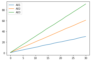
[3]:
fig, ax = pyplot.subplots()

for col in raw_data.columns:
    ax.plot(raw_data.index, raw_data[col], label=col)

ax.legend()
pyplot.show()
Creating murefi data structures
There are three types of data in murefi:
Timeseriesis just a pair of vectorstandy-Replicatebundles multipleTimeseriesinto one realization of an experiment -Datasetcontains manyReplicatesthat are all independent of each other
With these data structures, every single measurement can (and should!) have its own timestamp. Also, all the Timeseries may have different lengths.
Now let’s assume that the raw_data from above are trajectories of absorbance-values for three Replicates.
[4]:
dataset = murefi.Dataset()

# make a replicate for each well
for well in raw_data.columns:
    # create a Replicate object and name it after the well
    rep = murefi.Replicate(rid=well)
    # then fill it with the timeseries
    rep['A430'] = murefi.Timeseries(
        t=numpy.array(raw_data.index),
        y=numpy.array(raw_data[well]),
        # independent_key describes the dimension (e.g. X, S, P, acid, ...)
        # the dependent key is usually the unit of measurement
        independent_key='P', dependent_key='A430'
    )
    # add variable-length glucose data
    n = numpy.random.randint(5, 30)
    rep['glc'] = murefi.Timeseries(
        t=numpy.arange(0, n),
        y=30-numpy.random.normal(numpy.arange(0, n), scale=.2),
        independent_key='S',
        dependent_key='glc'
    )
    # finally, add the replicate to the dataset
    dataset[rep.rid] = rep

# by just printing out the dataset, its contents are summarized:
dataset
[4]:
Dataset([('A01', Replicate(A430[:20], glc[:18])),
         ('A02', Replicate(A430[:20], glc[:27])),
         ('A03', Replicate(A430[:20], glc[:5]))])
Using the data structures
Dataset and Replicate are dictionaries. They can be indexed with [key] and iterated over using .items():
[5]:
for rid, replicate in dataset.items():
    print(f'Replicate "{rid}" contains timeseries for: {set(replicate.keys())}')
Replicate "A01" contains timeseries for: {'glc', 'A430'}
Replicate "A02" contains timeseries for: {'glc', 'A430'}
Replicate "A03" contains timeseries for: {'glc', 'A430'}
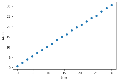
[6]:
rep_A01 = dataset['A01']
A430_A01 = rep_A01['A430']

fig, ax = pyplot.subplots()

ax.set_xlabel('time')
ax.set_ylabel(A430_A01.dependent_key)
ax.scatter(A430_A01.t, A430_A01.y)

pyplot.show()
Saving and loading datasets
A murefi.Dataset can be saved to and loaded from a HDF5 file as shown below:
[7]:
dataset.save('Test123.h5')
[8]:
murefi.load_dataset('Test123.h5')
[8]:
Dataset([('A01', Replicate(A430[:20], glc[:18])),
         ('A02', Replicate(A430[:20], glc[:27])),
         ('A03', Replicate(A430[:20], glc[:5]))])
[9]:
%load_ext watermark
%watermark -n -u -v -iv -w
Last updated: Mon Mar 29 2021

Python implementation: CPython
Python version       : 3.7.9
IPython version      : 7.19.0

pandas    : 1.2.1
numpy     : 1.19.2
matplotlib: 3.3.2
murefi    : 5.0.0

Watermark: 2.2.0